Document Comparison & Visualization
LocalVectorDB includes built-in methods for comparing documents at the document and chunk level, finding nearest neighbours, computing pairwise similarity matrices, and visualising the embedding space.
Document-Level Comparison
Comparing Two Documents
Use compare_documents() to get the cosine similarity (normalised to [0, 1]) between two
documents based on their centroid embeddings:
score = db.compare_documents("doc_a", "doc_b")
print(f"Similarity: {score:.3f}")
A score of 1.0 means the documents are identical in embedding space; 0.5 means they are orthogonal; values approaching 0.0 mean they are as dissimilar as possible.
Finding Nearest Neighbours
nearest_neighbors() returns the k most similar documents to a reference document,
excluding the reference itself:
results = db.nearest_neighbors("doc_a", k=5)

for r in results:
    print(f"  {r.id}: {r.score:.3f}")
Results are QueryResult objects with type="document", sorted by score descending.
Note
This capability is also available outside the Python API: the CLI exposes it as
lvdb db <name> related <doc_id> (see Command-Line Interface) and the MCP server as the
find_related_documents tool (see MCP Server).
With filtering and thresholds:
results = db.nearest_neighbors(
    "doc_a",
    k=5,
    score_threshold=0.5,               # minimum similarity to include
    filters={"category": "research"},   # metadata filter
)
Pairwise Similarity Matrix
Compute an NxN similarity matrix for all (or selected) documents:
# All documents
matrix = db.pairwise_similarity_matrix()

# Selected subset
matrix = db.pairwise_similarity_matrix(doc_ids=["doc_a", "doc_b", "doc_c"])
The returned DocumentSimilarityMatrix contains:
matrix–np.ndarrayof shape (N, N) with pairwise similarity scoresdoc_ids– list of document IDs matching rows and columnsembeddings–np.ndarrayof shape (N, D), the document embeddings used
print(matrix.doc_ids)   # ['doc_a', 'doc_b', 'doc_c']
print(matrix.matrix)    # (3, 3) numpy array
Chunk-Level Comparison
compare_documents_detailed() reveals where two documents overlap and where they diverge
by aligning individual chunks:
result = db.compare_documents_detailed("doc_a", "doc_b", chunk_threshold=0.7)

print(f"Overall similarity: {result.overall_similarity:.3f}")
print(f"Matched in doc_a:   {result.matched_ratio_1:.1%}")
print(f"Matched in doc_b:   {result.matched_ratio_2:.1%}")

for a in result.chunk_alignments:
    print(f"  chunk {a.chunk_index_1} <-> chunk {a.chunk_index_2}: {a.similarity:.3f}")

print(f"Unmatched in doc_a: {result.unmatched_chunks_1}")
print(f"Unmatched in doc_b: {result.unmatched_chunks_2}")
How to interpret the result:
Scenario |
overall_similarity |
matched_ratio |
Interpretation |
|---|---|---|---|
Near-identical |
High (~0.9+) |
High (~1.0) |
Documents are very similar throughout |
Shared section |
Moderate (~0.6) |
Low (~0.3) |
Some shared content, mostly different |
Completely different |
Low (~0.3) |
~0.0 |
No meaningful overlap |
The chunk_threshold parameter controls the minimum similarity for a chunk pair to count
as “matched”.
Chunk Similarity Matrix
Where compare_documents_detailed() reduces each chunk to its single best match,
chunk_similarity_matrix() returns the full chunk-level pairwise similarity matrix.
This is the raw data behind the synteny and chord diagrams below, and is useful when you
want to inspect every chunk pair yourself.
# Cross-document: chunks of doc_a (rows) vs chunks of doc_b (columns)
cm = db.chunk_similarity_matrix("doc_a", "doc_b")

print(cm.matrix.shape)         # (C1, C2)
print(cm.chunk_indices_1)      # chunk indices for the rows
print(cm.chunk_indices_2)      # chunk indices for the columns
When doc_id_2 is omitted it defaults to doc_id_1, producing the (symmetric) self-similarity matrix of a single document – the input a chord diagram expects:
# Self-similarity within one document
cm = db.chunk_similarity_matrix("doc_a")
print(cm.doc_id_1 == cm.doc_id_2)   # True
Both documents must have chunk embeddings; a ValueError is raised otherwise.
Data Classes
from localvectordb.core import (
    ChunkAlignment,
    ChunkSimilarityMatrix,
    DocumentComparisonResult,
    DocumentSimilarityMatrix,
)
ChunkAlignment–chunk_index_1,chunk_index_2,similarityChunkSimilarityMatrix–matrix(shape(C1, C2)),doc_id_1,doc_id_2,chunk_indices_1,chunk_indices_2DocumentComparisonResult–doc_id_1,doc_id_2,overall_similarity,chunk_alignments,matched_ratio_1,matched_ratio_2,unmatched_chunks_1,unmatched_chunks_2DocumentSimilarityMatrix–matrix,doc_ids,embeddings
Visualization
The visualization module provides dimensionality reduction, clustering, and plotting utilities for exploring the document embedding space.
Installation
Visualization requires optional dependencies:
# Core visualization (scikit-learn + matplotlib)
pip install "localvectordb[visualization]"

# Interactive plots (adds plotly)
pip install "localvectordb[visualization-interactive]"
Gallery
Every figure below is real output from the functions documented on this page, over a real
corpus: 60 papers from the Qasper dev split (NLP papers
with their full text and native section structure), chunked by the shipped chunker and
encoded with embeddinggemma:300m. Nothing is synthetic or hand-tuned.
They are regenerated by benchmarks/doc_figures.py, which reads the embedding cache the
retrieval experiments already built, so reproducing the gallery costs no API calls:
./.venv/Scripts/python.exe -m benchmarks.doc_figures
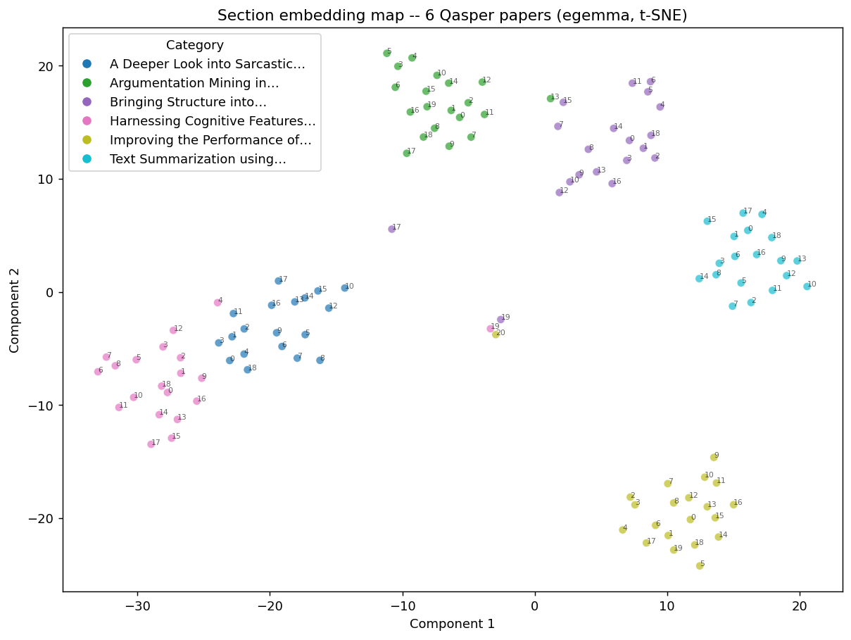
Embedding map. Each point is a section, coloured by the paper it came from. Nothing tells the projection which sections share a parent – the islands are the embedding space recovering document structure on its own.
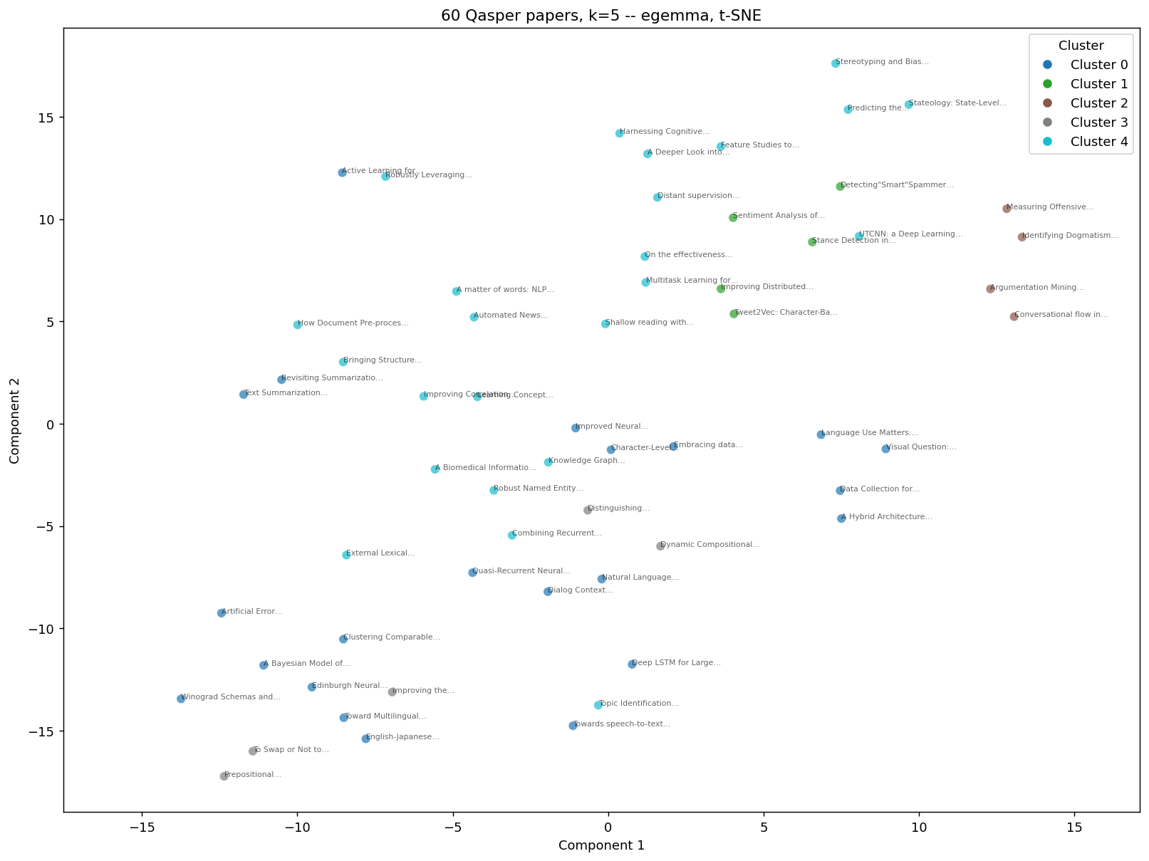
Clusters. All 60 papers at k=5, labelled by title. The groups are readable ones: Twitter and social-media representation, argumentation and online discourse, lexical semantics and syntax, and a larger core-NLP remainder.
Worth knowing before you trust an automatic k here:
find_optimal_clusters() picks 2 on this corpus, and silhouette
scores are low at every k (peak 0.076). That is the honest signal for a single-domain
collection – these papers form a gradient, not disjoint topics – and it is why this figure sets
k explicitly rather than taking the silhouette optimum at face value. On a corpus with genuinely
separable topics the automatic choice is far more useful.
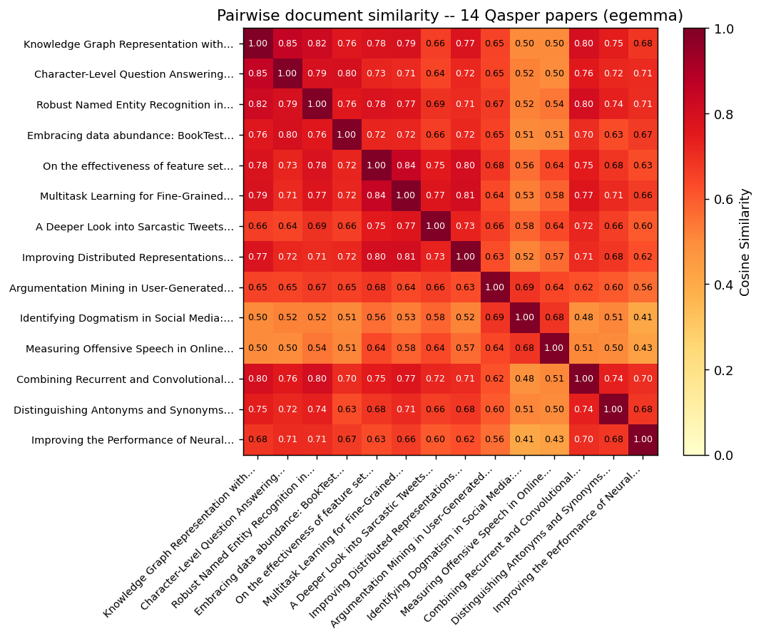
Pairwise similarity heatmap. Fourteen papers, drawn evenly from four k-means topic clusters and ordered by cluster so the block structure lands on the diagonal. Cells are annotated automatically below 20 documents.
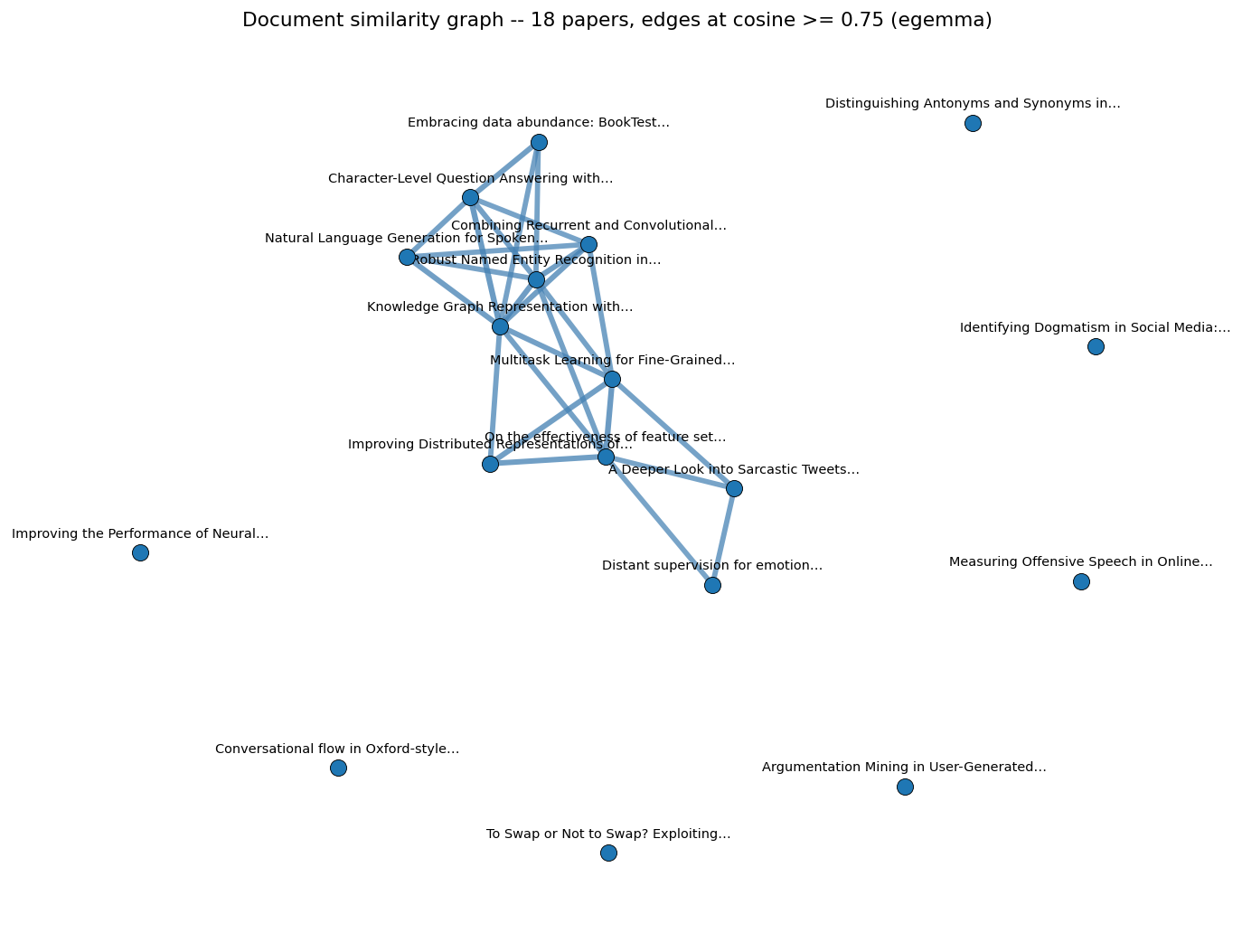
Similarity graph. Eighteen papers as nodes, with an edge wherever cosine similarity clears
0.75 (the top ~18% of pairs). Edge width and opacity scale with similarity. The default
layout="spring" runs a force-directed layout over the thresholded edges, so the connected
component pulls together into one visible group. Isolated nodes are real: they are the papers
with no close neighbour in this slice, and the layout pushes them out to the rim rather than
leaving them mixed in.
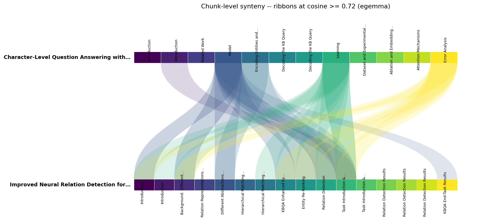
Synteny. Two related papers – character-level question answering and neural relation
detection – drawn as chunk tracks with ribbons between similar chunks. Each segment is labelled
with the section it falls in (via labels_1/labels_2) rather than a bare index, so the
ribbons can be read directly: Introduction to Introduction, Model to Different
Abstractions, Error Analysis to KBQA End-Task Results.
Choosing a threshold matters here: two papers on adjacent topics are broadly similar everywhere, so a permissive threshold fills the panel with a wash. At the top ~12% of chunk pairs the surviving ribbons are the real correspondences.
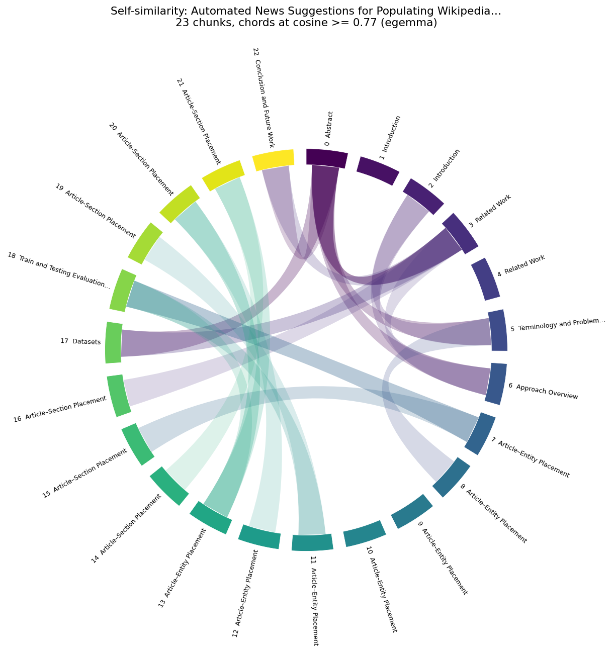
Chord. A single paper’s internal self-similarity across its 23 chunks, with
min_chunk_distance=3 suppressing the trivially-similar neighbours. Arcs carry the section
each chunk belongs to (via labels), which turns the diagram from “chunk 17 resembles chunk 3”
into something you can act on: the Article-Entity Placement chunks bind to each other across
the whole paper, and Abstract reaches all the way round to Related Work.
Comparing Embedding Models
Because these plots take embeddings rather than a provider, the same corpus can be run through different encoders and compared directly – a practical way to decide what to index with.
Below are the same 30 papers under four encoders. Each panel is an independent PCA of that
model’s own vectors; the colours are held fixed at embeddinggemma’s k-means labels
(k=4), so a panel that keeps its colours separated is an encoder that agrees about which
papers belong together.
Three questions are overlaid as large markers. Each is embedded by that panel’s model, with that model’s query prefix, then projected into the same space – so the figure shows where each encoder puts a question relative to the documents that answer it. Document dot size scales with relevance to the queries.
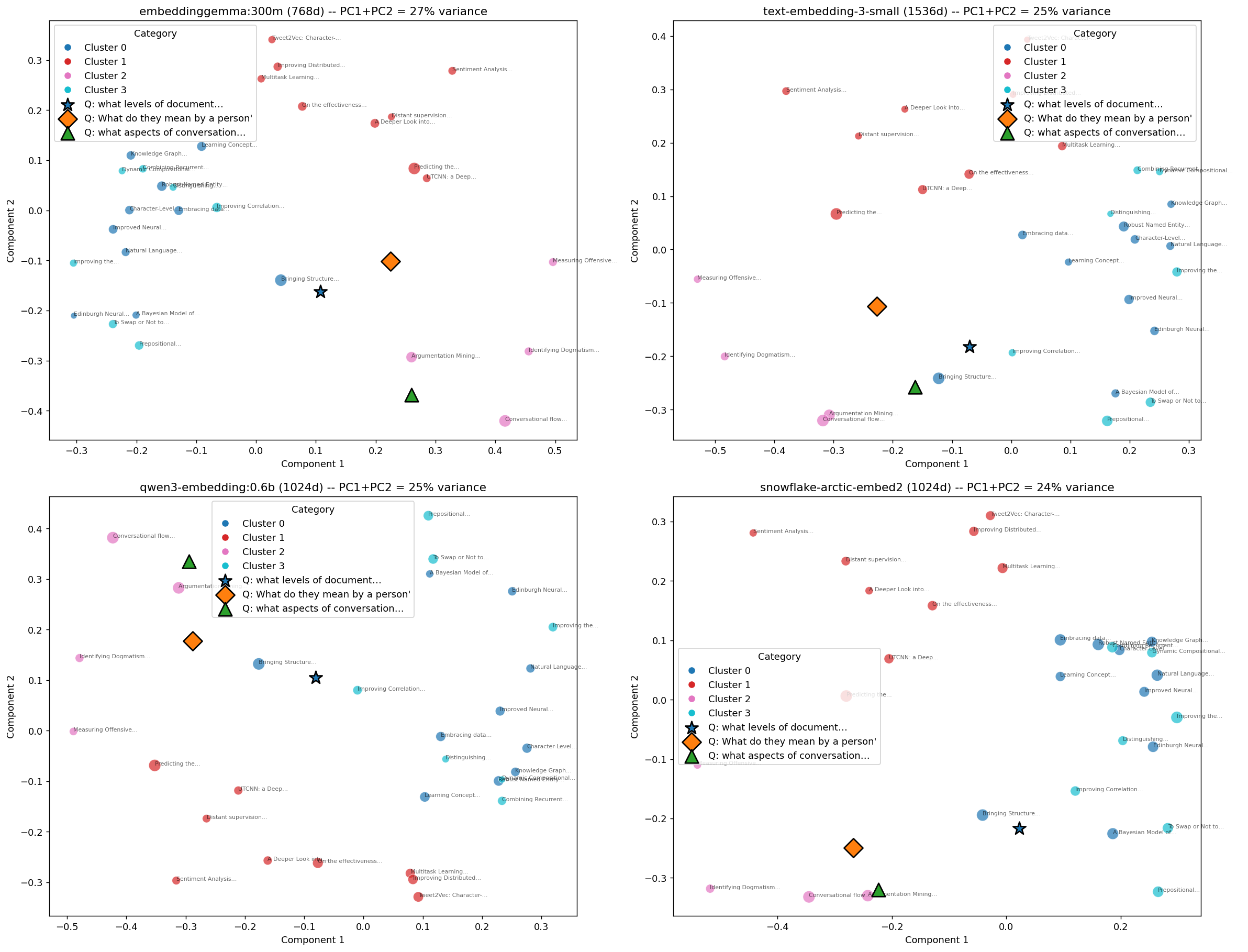
Read the grouping, not the orientation. The sign and order of principal components are arbitrary, so panels are rotated and mirrored relative to one another for reasons that carry no meaning. What does carry meaning is that the clusters stay coherent in all four; that every model drops “what aspects of conversation flow do they look at?” next to Conversational flow in Oxford-style debates and Argumentation Mining; and that the 1536-dimension OpenAI model buys no visibly cleaner separation than the 768-dimension local one.
The queries were picked for being specific. Qasper is full of questions like “What baselines are used for comparison?”, which apply to every paper in the corpus and duly embed to the middle of the space, overlaying nothing useful – a good reminder that a query overlay is only as informative as the query.
To put a number on that, correlate each model’s full document-by-document similarity profile with every other model’s:
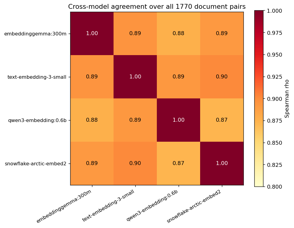
All four agree closely (Spearman rho 0.87–0.90 over all 1,770 document pairs). For
document-level structure on this corpus the choice of encoder is close to a wash – which is
worth knowing before paying for the larger model. Retrieval quality is a different question,
measured against benchmarks/RETRIEVAL_BASELINE.md, and it does separate these models.
Convenience Methods
The database object provides several high-level methods that handle embedding extraction, projection, and plotting in a single call.
Embedding map:
# 2D scatter plot of all documents
fig = db.visualize_documents(method="tsne")
fig.savefig("embedding_map.png")

# Colour by a metadata field
fig = db.visualize_documents(method="pca", color_by="category")

# Cluster and colour by cluster
fig = db.visualize_documents(method="tsne", n_clusters=4)

# Interactive plotly plot
fig = db.visualize_documents(method="pca", interactive=True)
fig.show()
Query overlay:
Show how query strings relate to the document space. Query points are projected into the same 2D space and displayed as distinct markers. Document dot sizes scale by relevance to the queries.
fig = db.visualize_queries(
    queries=["web development", "neural networks"],
    method="pca",
)
Synteny ribbon diagram:
Compare two documents chunk-by-chunk as a synteny plot: each document is drawn as a track of chunk segments, and ribbons connect similar chunks between them. This makes reordered, inserted, or shared passages easy to spot at a glance.
# Ribbons drawn only for chunk pairs at or above the similarity threshold
fig = db.visualize_synteny(
    "doc_a",
    "doc_b",
    similarity_threshold=0.7,
    orientation="horizontal",   # or "vertical"
    chunk_labels=True,           # annotate each segment with its chunk index
)
fig.savefig("synteny.png")

# Label segments with anything you like instead of the index -- one entry per
# chunk, per document. Text labels are drawn outside the track, since a
# heading does not fit inside a segment the way a numeral does.
fig = db.visualize_synteny(
    "doc_a",
    "doc_b",
    labels_1=["Introduction", "Method", "Results"],
    labels_2=["Background", "Approach", "Evaluation"],
)

# Interactive plotly version -- labels work here too, and also appear in the
# hover text for each segment
fig = db.visualize_synteny("doc_a", "doc_b", labels_1=[...], interactive=True)
fig.show()
Chord diagram:
Visualise a single document’s internal structure as a Circos-style chord diagram. Chunks are placed around a circle and chords link chunks that are similar to one another, revealing repetition and long-range self-reference within the document.
fig = db.visualize_chord(
    "doc_a",
    similarity_threshold=0.7,
    min_chunk_distance=3,   # ignore chords between chunks fewer than 3 apart
    chunk_labels=True,
)
fig.savefig("chord.png")

# Name the arcs instead of numbering them -- one entry per chunk. Text labels
# are rotated to follow the circle, so long names stay legible.
fig = db.visualize_chord("doc_a", labels=["Abstract", "Introduction", "Method"])

# Interactive plotly version -- labels work here too, and also appear in the
# hover text for each arc
fig = db.visualize_chord("doc_a", labels=[...], interactive=True)
fig.show()
The min_chunk_distance parameter suppresses chords between neighbouring chunks (which are
almost always similar), keeping the plot focused on meaningful long-range connections.
Standalone Visualization API
For more control, use the visualization module directly.
Dimensionality reduction:
from localvectordb.visualization import reduce_dimensions

# PCA
projection = reduce_dimensions(embeddings, method="pca", doc_ids=ids)
print(projection.coordinates.shape)     # (N, 2)
print(projection.explained_variance)    # variance ratio per component

# t-SNE
projection = reduce_dimensions(embeddings, method="tsne", doc_ids=ids)
reduce_dimensions() returns an EmbeddingProjection containing coordinates, the
fitted transformer (for projecting new points), and document IDs.
Clustering:
from localvectordb.visualization import cluster_embeddings, find_optimal_clusters

# Auto-detect optimal k via silhouette analysis
k = find_optimal_clusters(embeddings)
clusters = cluster_embeddings(embeddings, n_clusters=k)

print(clusters.labels)      # (N,) cluster assignments
print(clusters.centroids)   # (K, D) cluster centres
print(clusters.n_clusters)  # K
Plotting:
from localvectordb.visualization import (
    plot_embedding_map,
    plot_similarity_matrix,
    plot_clusters,
    plot_similarity_graph,
)

# Scatter plot
fig = plot_embedding_map(projection, color_by=labels)

# Similarity heatmap
matrix = db.pairwise_similarity_matrix()
fig = plot_similarity_matrix(matrix)

# Cluster plot
fig = plot_clusters(projection, clusters)

# Similarity graph (nodes = docs, edges = similarity above threshold)
fig = plot_similarity_graph(matrix, threshold=0.5)

# layout="spring" (the default) is a force-directed layout over the edges that
# survived the threshold: connected documents group, unconnected ones move to
# the rim. layout="mds" instead embeds the *full* similarity matrix, placing
# every document by its distance to every other whether or not an edge is drawn.
fig = plot_similarity_graph(matrix, threshold=0.5, layout="mds")
Two knobs trade legibility against contrast in the spring layout, and both are forwarded from
plot_similarity_graph: gravity pulls nodes toward the centre (without it, unconnected
nodes accelerate off to the rim and flatten everything else into the middle), and spread
multiplies the ideal edge length. The defaults loosen a densely connected component enough that
node labels stay readable; lower them for maximum contrast between clusters, raise them further
and the clustering starts to wash out.
Graph structure (for custom processing):
from localvectordb.visualization import build_similarity_graph

graph = build_similarity_graph(matrix, threshold=0.4)
# graph["nodes"] = [{"id": "doc_a", "index": 0}, ...]
# graph["edges"] = [{"source": "doc_a", "target": "doc_b", "weight": 0.82}, ...]
Interactive plots (plotly):
from localvectordb.visualization import (
    plot_embedding_map_interactive,
    plot_similarity_matrix_interactive,
)

fig = plot_embedding_map_interactive(projection)
fig.show()

fig = plot_similarity_matrix_interactive(matrix)
fig.show()
Common Patterns
Finding Duplicate Documents
matrix = db.pairwise_similarity_matrix()

for i in range(len(matrix.doc_ids)):
    for j in range(i + 1, len(matrix.doc_ids)):
        if matrix.matrix[i, j] >= 0.95:
            print(f"Duplicate: {matrix.doc_ids[i]} <-> {matrix.doc_ids[j]}")
Topic Clustering
from localvectordb.visualization import cluster_embeddings, find_optimal_clusters

# pairwise_similarity_matrix() returns the document embeddings and IDs for all
# documents (pass doc_ids=[...] to restrict to a subset).
matrix = db.pairwise_similarity_matrix()
embeddings, doc_ids = matrix.embeddings, matrix.doc_ids
k = find_optimal_clusters(embeddings)
clusters = cluster_embeddings(embeddings, n_clusters=k)

for cid in range(clusters.n_clusters):
    members = [doc_ids[i] for i, l in enumerate(clusters.labels) if l == cid]
    print(f"Cluster {cid}: {members}")
Content Gap Analysis
Use detailed comparison to find what was added between document versions:
result = db.compare_documents_detailed("doc_v1", "doc_v2", chunk_threshold=0.6)

if result.unmatched_chunks_2:
    doc = db.get("doc_v2")
    # db.get() returns document content/metadata only; re-derive the chunks
    # (with their indices) using the database's chunker.
    chunks = db.chunker.chunk(doc.content)
    print("New content in v2:")
    for chunk in chunks:
        if chunk.index in result.unmatched_chunks_2:
            print(f"  [{chunk.index}] {chunk.content[:100]}...")